3.7 Using scoring and non-scholarly text
The text visualizations in VOSviewer are well worth using in analyses that are not about scholarly literature per se. In fact you can analyze phrases in any text document, as long as the text is presented to VOSviewer in English (the algorithm is only trained in English grammar).
The use of scoring files makes analysis with VOSviewer much more interesting. For example it allows us to visualize if articles contain a specific word, author or topic and see what effect this has on the mapping. One example where such an analysis may be helpful, is when you doubt the specific scholarly term for a subject (jargon). In multidisciplinary research you may find that the terms are used by different groups. By overlaying the occurrence of this term in combination with other terms, you will find out which one best suits your article.
In this analysis we chose to start from a different situation in which we analyze news articles written about Leiden University and indexed in Nexis Uni. As these articles are in Dutch we had to translate them to English first with DeepL. Next we applied scoring to the different newspapers: does a local newspaper write about different subjects than a national one? Or than a religiuous one?
For this analysis we have written Python code. The code can be copied by clicking the button at the right top of the code box.
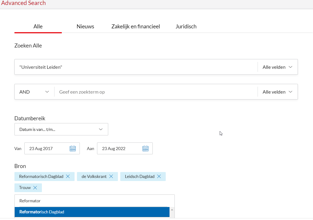
- Go to Nexis Uni, change to ‘Advanced Search’ and search for “Universiteit Leiden” . We set the filters to include only the following newspapers: Volkskrant, Trouw, Leidsch Dagblad en Reformatorisch Dagblad for the period 23-08-2017 until 23-08-2022.
img
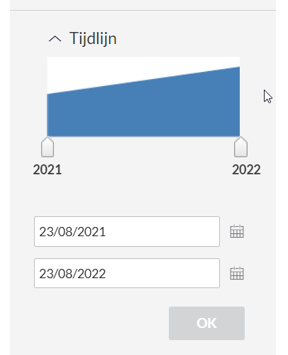
- We want to export all articles as full text, preferrably in .rtf as this can be read easily by Python. We can only do this if we break down our search in smaller numbers of articles, as we are allowed to export only the first 1000 results. So filter year by year and export in these subsets by first going to ‘Tijdlijn’ in the left column and then setting the timeline so you will have less than 1000 results.
img
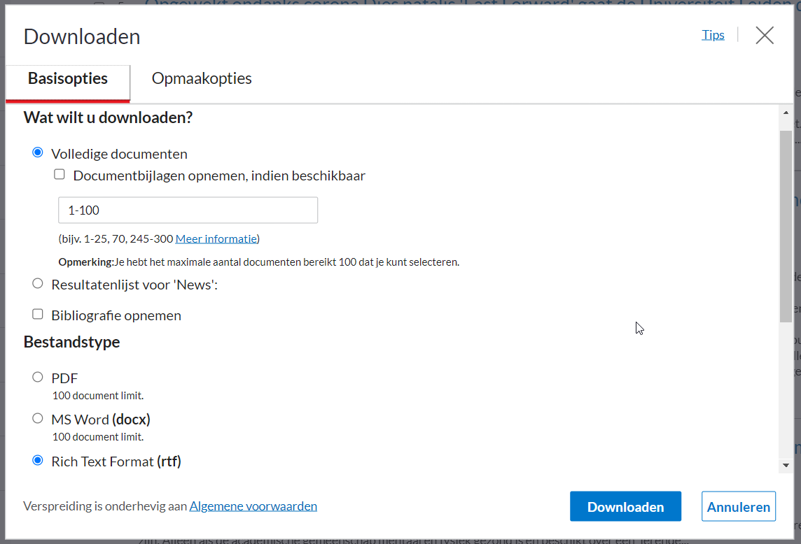
- Click on the download button at the top (arrow down) and use the settings below. As downloading functions for sets of 100, you have to fill out the field ‘Volledige documenten’ to the document numbers in the set and repeat this action until all documents have been downloaded. Make sure you save all documents in the same directory.
img
- Next we will write Python code to create text files for VOSviewer to work with. We start with creating the necessary text files and importing the libraries needed to convert the works. There is also some code to make sense of the way in which Nexis Uni describes it’s articles as we need to convert them to something that makes sense to VOSviewer.
from striprtf.striprtf import rtf_to_text
from datetime import date
import re
import os

#this file contains the text we want to analyze
text_file = open("all_text.txt", "w+", encoding="utf-8")

#this is our scoring file
metadata_file = open("metadata.txt", "w+", encoding="utf-8")

#this function converts the date format in Nexis Uni to normal dates
def get_days(date_article, corr_date):
    # translate dutch date into number of days
    # dag maand jaar weekdag
    date_parts = date_article.split(" ")
    day, month, year = 0, 0, 0
    if len(date_parts)>3:
        day = int(date_parts[0])
        year = int(date_parts[2])
        if date_parts[1]=='januari':
            month = 1
        elif date_parts[1]=='februari':
            month=2
        elif date_parts[1]=='maart':
            month=3
        elif date_parts[1]=='april':
            month=4
        elif date_parts[1]=='mei':
            month=5
        elif date_parts[1]=='juni':
            month=6
        elif date_parts[1]=='juli':
            month=7
        elif date_parts[1]=='augustus':
            month=8
        elif date_parts[1]=='september':
            month=9
        elif date_parts[1]=='oktober':
            month=10
        elif date_parts[1]=='november':
            month=11
        elif date_parts[1]=='december':
            month=12

    the_date = date(year, month, day)
    return (the_date-corr_date).days

#this function removes some common layout words in NexisUni
def remove_common(text_in):
    text_in = text_in.replace("Pdf", "")
    text_in = text_in.replace("van dit document", "")
    text_in = text_in.replace("document load date", "")
    text_in = text_in.replace("load date", "")
    text_in = text_in.replace("Medium", "")
    text_in = text_in.replace("Shading", "")
    text_in = text_in.replace("Grid", "")
    text_in = text_in.replace("Accent", "")
    text_in = text_in.replace("Pagina", "")
    text_in = text_in.replace("Light", "")
    text_in = text_in.replace("List", "")
    text_in = text_in.replace("Colorful", "")
    text_in = text_in.replace("Dark", "")
    text_in = text_in.replace("Subtle", "")
    text_in = text_in.replace("Emphasis", "")
    text_in = text_in.replace("Intense", "")
return text_in- The NexisUni export is quite uniform. We can readout the contents by checking all files in the directory we saved our rtf’s. Each file has metadata describing the article specifically structured (but a bit difficult to read for a script), something you will discover while looking at some examples. The title for example, is always after the url, and after the title we first have the news outlet and then the date. The document text is in between the line ‘Body’ and ‘End of document’.
for article in os.listdir('articles_nexisuni'): #read all files in the directory articles_nexisuni
    if article[:2]!="~$": # skip temporary files.
        news_article = open(os.path.join('articles_nexisuni', article), 'r', encoding="utf-8")
        i = 0
        next_section = ' '
        title = ''
        newspaper = ''
        article_date = ''
        body = ''
        for line in news_article.readlines():
            i+=1
            line=rtf_to_text(line, 'ignore')
            line = line.strip()
            if len(line)>0 and line!="":

                if line[:6]=="https:" and len(title)<=0:
                    next_section = 'title'
                elif next_section=='title':
                    if not (line=="de Volkskrant" or line=='Trouw' or line=='Leidsch Dagblad' or line=="Reformatorisch Dagblad"):
                        title += line
                    else:
                        newspaper = line
                        next_section = 'article_date'
                elif next_section=='article_date':
                    article_date = get_days(line, date(2017,8,23)) #we calculate the number of days since the first publication in our set
                    next_section = 'wait'
                elif next_section=='wait' and line[:4]=="Body":
                    next_section = 'body'
                elif next_section=='body' and not line[:15]=="End of Document":
                    body += line + " " + '\n'
                elif next_section=='body' and line[:15]=="End of Document":
                    next_section='end'

        #We have to strip all information from the body
        pattern = re.compile(r'[\n\r]+') #r'[^\w\.,;: ]+')
        body = title + " " + body
        body = re.sub(pattern, ' ', body)
        body = remove_common(body) # to remove some common nexis uni terms

        text_file.write(body+'\n')
        volkskrant, trouw, leidsch_dagblad, reformatorisch_dagblad, voermans = 0,0,0,0,0
        if newspaper =='de Volkskrant':
            volkskrant=1
        elif newspaper=='Trouw':
            trouw=1
        elif newspaper=='Leidsch Dagblad':
            leidsch_dagblad=1
        elif newspaper=='Reformatorisch Dagblad':
            reformatorisch_dagblad=1
        # let's do an extra check to see if Wim Voermans is involved
        if re.search("(?i)voermans", body, re.IGNORECASE):
            voermans=1
        metadata_file.write(f'\n{article_date}\t{volkskrant}\t{trouw}\t{leidsch_dagblad}\t{reformatorisch_dagblad}\t{voermans}')

# next we save and close the files
metadata_file.close()
text_file.close()- After the script has worked through all the files, we have a text file (all_text.txt) and a scoring file (metadata.txt). Entering these into VOSviewer would give unusable results as the VOSviewer algorithm can only work with English phrases. Therefore we have to translate the text.
In theory translation can be done in several ways, for example by using Google Translate API. However, the sheer size of the text (we are indexing fulltext!) means this would cost us upwards of 100 dollars. A cheaper way is to take a test or full subscription to DeepL and convert text files. You can take out a DeepL trial or subscription at https://www.deepl.com/ (for smaller searches this may work well without subscription). For DeepL the maximum text size is 1 Mb, so our first step is to split the text files:
def split_into_files(text_size_limit=800000):
    text_size_counter = 0
    file_number = 0
    with open("all_text.txt", encoding="utf-8") as f:
        lines = f.readlines()
        current_file = open("all_text_"+str(file_number)+".txt", "w+", encoding="utf-8")
        for line in lines:
            text_size_counter += len(line)+2 #add linebreaks as character
            if text_size_counter > text_size_limit:
                current_file.close()
                file_number += 1
                current_file = open("all_text_"+str(file_number)+".txt", "w+", encoding="utf-8")
                text_size_counter = len(line)+2
            current_file.write(line)
        current_file.close()

split_into_files()- The split files can be uploaded to DeepL and after that we can stitch the results back to one big file (be sure to keep the same order of the files, otherwise the scoring file will be off). We can do this with the following script:
def combine_files(name="all_text_"):
    # walk the os_path
    file_names_found = {}
    full_translation = open("all_text_translated.txt", "w+", encoding="utf-8")
    for x in os.listdir():
        print(x)
        if x.find(name) >= 0:
            pattern = re.compile('_([0-9]+) ')
            pos = pattern.search(x)
            if pos:
                print("pos: "+ pos.group(1))
                file_names_found[int(pos.group(1))] = x
    # start retrieving files
    for i in range(0, len(file_names_found)):
        with open(file_names_found[i], encoding="utf-8") as f:
            for line in f.readlines():
                if line.strip() != "": #remove empty last lines
                    full_translation.write(line)
            f.close()
    full_translation.close()
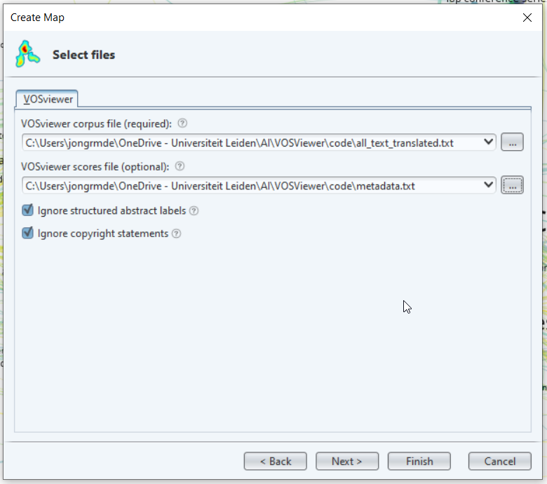
combine_files()- Now we can use VOSviewer to create a plot with multiple overlays. Choose ‘Create’->‘Create a map based on text data’->‘Read data from Vos Viewer files’. Use the first file box for the text file and the second one for the scoring file.
img
In the next window we choose binary counting. In this case we don’t use a thesaurus, but if you want to ensure that certain synonyms are grouped together, you can use a thesaurus.
When asked for a minimum number of terms I usually select to keep around the 1000-2000 results. In this case this means a term should occur at least 24 times. Next we finish and create our map.
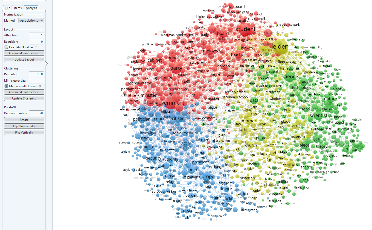
img
- Looking at our map, I get the idea that some clusters are overlapping too much. In red, for example, I see both students and political parties mentioned. Therefore it may be better to increase the resolution and create more clusters. To do this I have entered 1.2 in the box for resolution (Analysis tab on the left side, see Clustering). Press ‘Update clustering’ to create the new visualization.
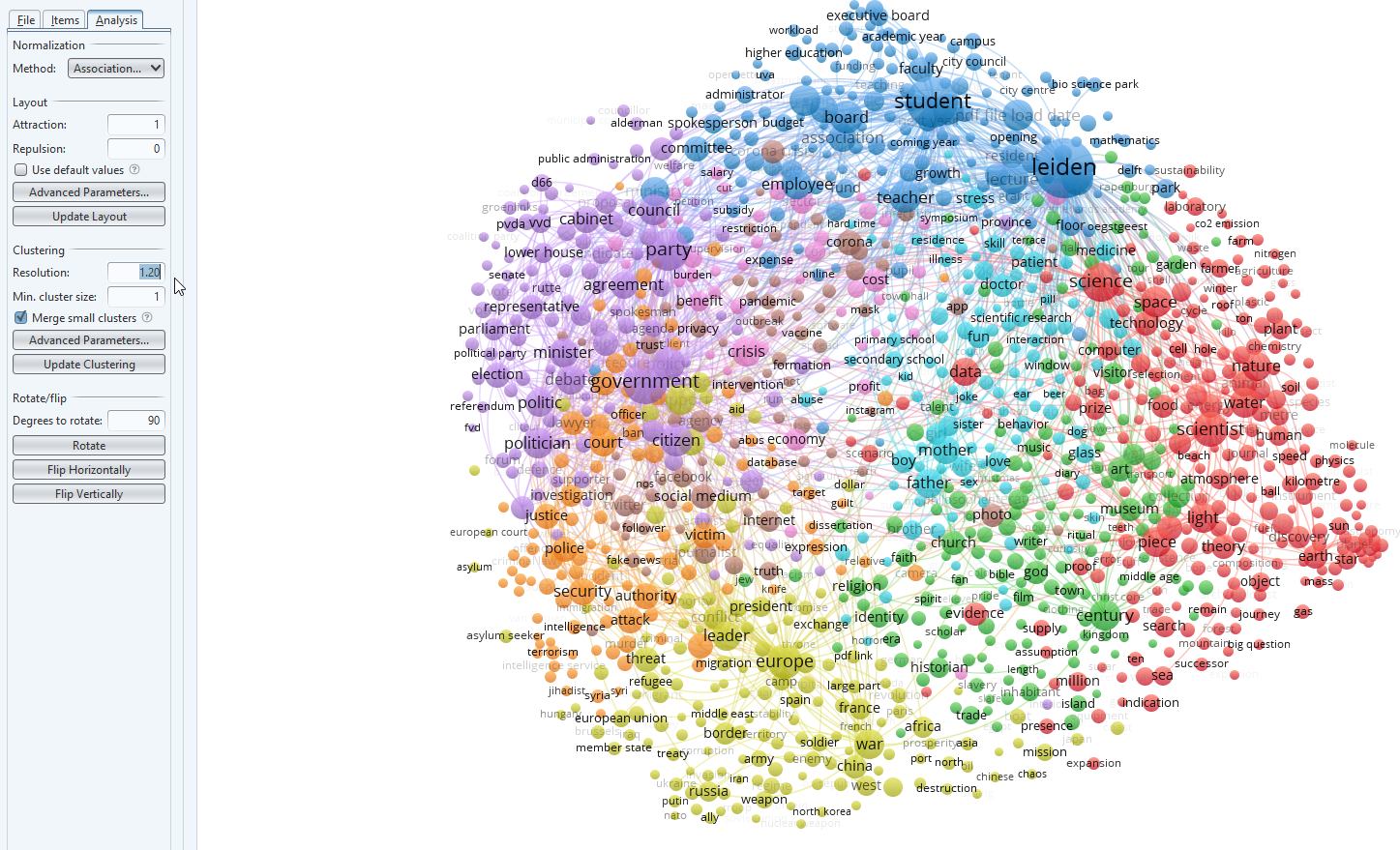
img
- The clusters are know separated in a more meaningful way. A quick look clockwise:
- blue (board, student, spokesperson, Leiden) seems to be about university affairs
- red (science, space, technology, computer, data) about scholarly output in the exact sciences
- green (Century, church, art, museum, visitor) this may well be connected to the Leiden past as we have had an anniversary during the analysis.
- yellow (Europe, leader, war, Russia) about international affairs
- orange (police, security, victim, court) about justice
- purple (government, party, citizen, politician) about politics
- light blue in the middle about family affairs/people
- Now we go to the tab ’Overlay visualization’at the top of VOSviewer. On the right we can choose what visualization we want. By default it uses the first score, in our case number of days since the start of the newsline. Under scores you can select the scoring you want to use, fo example our news source Volkskrant.
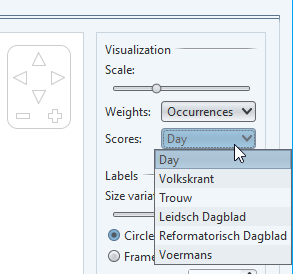
img
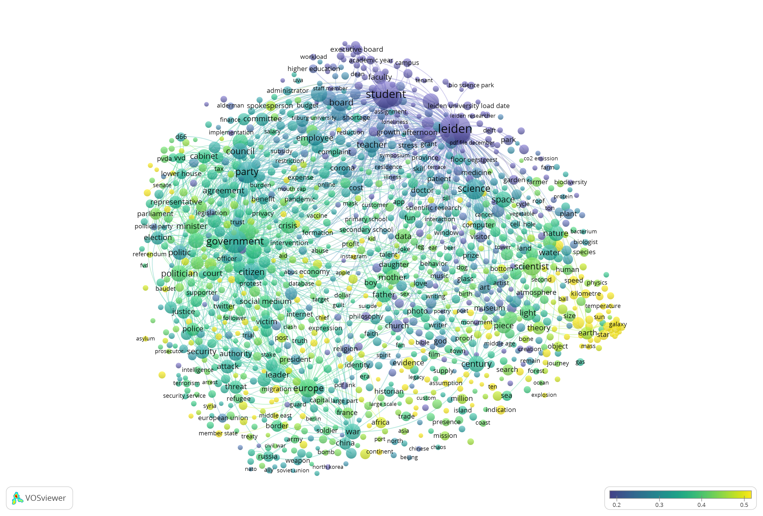
- Let’s switch to the scoring for ‘Wim Voermans’. Voermans is a well know Leiden professor of consitutional and administrative law. He is regularly asked for comments on state affairs, for example during the elections or for the nitrogen emission rights that have a large impact on the functioning of our government. The visualization reflects this. These topics (cabinet, council, debate, nitrogen) are yellow in the visualization (often occur in combination with Wim Voermans as you can see in the scale at the bottom). The size of the dot of each cluster, is an indication whether the topic is mentioned a lot within all documents.
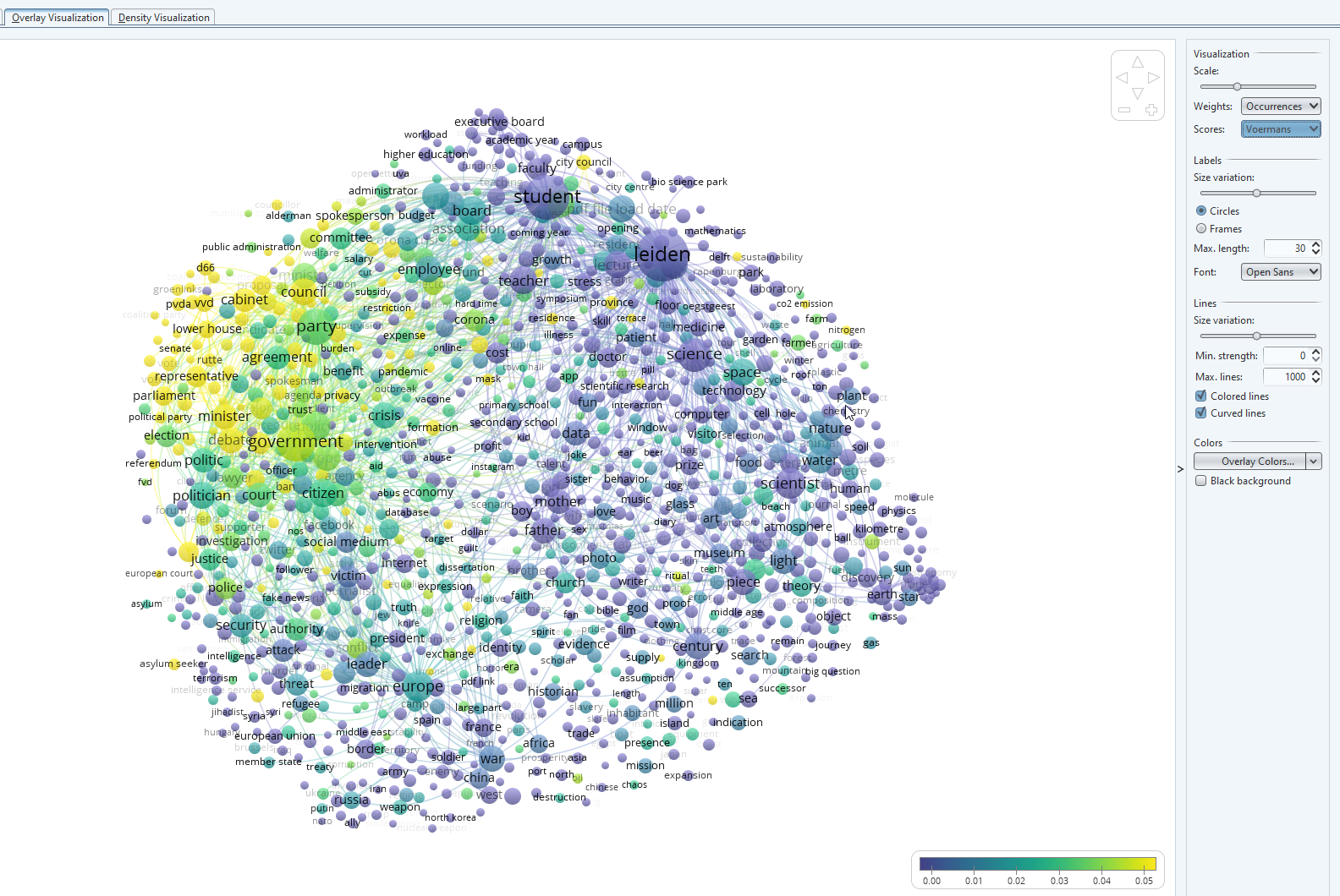
img
- For the newspapers ‘Trouw’, ‘De Volkskrant’, ‘Leidsch Dagblad’ and ‘Reformatorisch Dagblad’. These newspapers have been selected as they all have a different profile. The visualization gives information on how they differ from the average.
- Leidsch Dagblad is a local newspaper. In the visualization we can see it focuses (yellow). You can see it overlaps mainly with the university affairs cluster with words like campus being mentioned a lot) we saw earlier. There is not that much focus on the other topics such as science or state affairs. If we hover over the word ‘campus’ you will see a score in the bottom bar for Leidsch Dagblad of 0.74. This means that for the 86 occurrences of ‘campus’ in the set, 74 per cent - 64 - times it was in Leidsch Dagblad. So even though the number of occurrences is relatively small, the use of the term is quite unique for Leidsch Dagblad thus it has a specific focus here. (If all newspapers found it of equal interest, it would have been around 0.2-0.3 and blue)

img

img
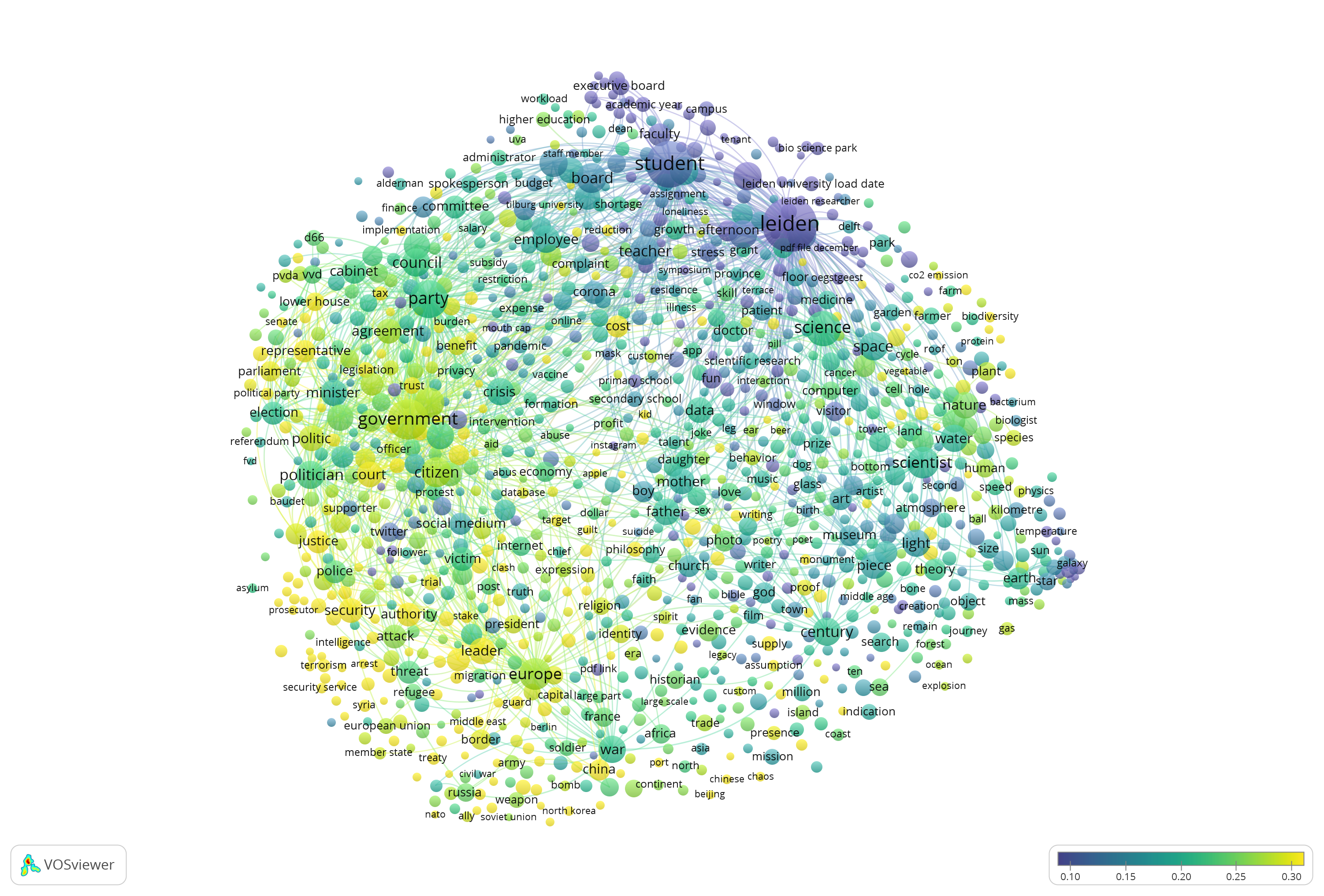
- De Volkskrant is a big national newspaper, a bit elitist and it is well known for politics and science reporting. You can immediately see that within this set Volkskrant is dominant in reporting about our observatory, while the university affairs are less important. (Be aware that Leidsch Dagblad has a dominance in university affairs, but even then, Volkskrant scores 0.13 while we expected 0.25 according to the table below).
img
- Trouw is a modern christian newspaper well known for reporting science and high quality journalism. It’s a bit of a generalist in this set. It’s not doing that well in astronomy which is a subject that may question belief. Within the set its focus is slightly more towards politics, security and international relations.
img
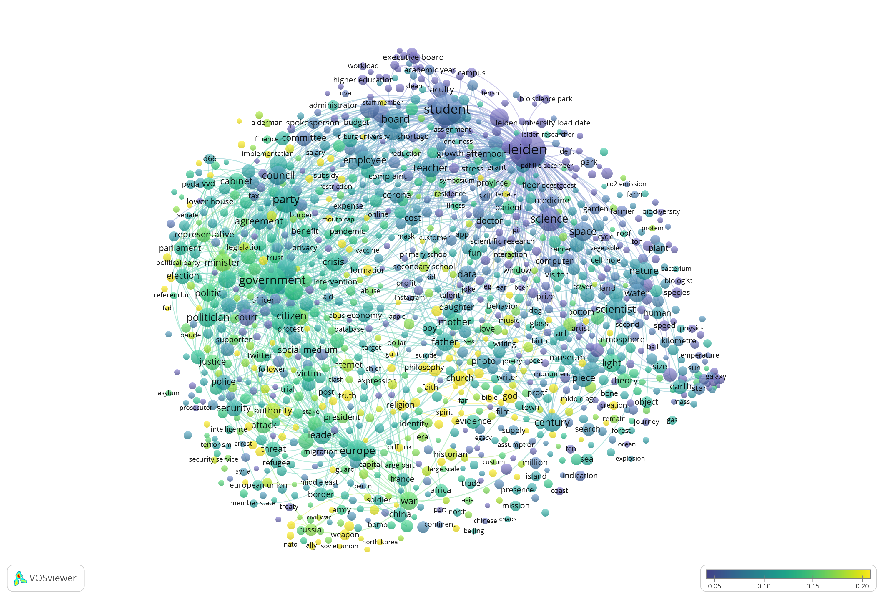
- Reformatorisch Dagblad is a very traditional christian newspaper. Judging by the scale, it is pretty average in most subjects. Within the set it has a focus on for example words such as god (0.42) and church (0.39). This is remarkable as the number of articles from this source is lower than from the other sources.
img
| Source | # documents | Average |
|---|---|---|
| De Volkskrant | 794 | 0.25 |
| Leidsch Dagblad | 1637 | 0.49 |
| Reformatorisch Dagblad | 321 | 0.10 |
| Trouw | 589 | 0.18 |